Regular Expressions

상위 문서: Regular Languages

개요

정규 표현식(regular expression)은 문자열에서 특정한 패턴을 찾거나 치환·검증하기 위해 사용하는 표현식이다.

Formal Definition of Regular Expressions

정규 표현식 집합 [math]\displaystyle{ \mathcal{RE} }[/math]는 알파벳 집합 [math]\displaystyle{ \Sigma }[/math]에 대해 아래의 닫힘 조건(closure conditions)을 만족하는 최소 집합을 의미한다:

1. [math]\displaystyle{ a \in \mathcal{RE},\,\, \forall a \in \Sigma }[/math]
2. 빈 문자열 [math]\displaystyle{ \epsilon }[/math]에 대해, [math]\displaystyle{ \epsilon \in \mathcal{RE} }[/math]
3. 어떤 문자열도 포함하지 않는 공집합 [math]\displaystyle{ \empty }[/math]에 대해, [math]\displaystyle{ \empty \in \mathcal{RE} }[/math]
4. Union: If [math]\displaystyle{ R_1 \in \mathcal{RE}, R_2 \in \mathcal{RE} }[/math], then [math]\displaystyle{ (R_1 \cup R_2) \in \mathcal{RE} }[/math]
5. Concatenation: If [math]\displaystyle{ R_1 \in \mathcal{RE}, R_2 \in \mathcal{RE} }[/math], then [math]\displaystyle{ (R_1 \circ R_2) \in \mathcal{RE} }[/math]
6. Kleene Star: If [math]\displaystyle{ R_1 \in \mathcal{RE} }[/math], then [math]\displaystyle{ (R_1*) \in \mathcal{RE} }[/math]

이때 정규 표현식은 단순히 문자열(strings)이며, [math]\displaystyle{ \{\empty, \epsilon, (, ), \cup, \circ, *\} \cup \Sigma }[/math]라는 알파벳 집합 위에서 정의된다. 따라서, [math]\displaystyle{ a \cup b }[/math]라는 정규표현식이 문자열로 해석되어 단순히 알파벳 [math]\displaystyle{ a,\cup,b }[/math]의 조합인지, 혹은 정규표현식 [math]\displaystyle{ a, b }[/math]의 합집합으로 해석되는지는 맥락에 따라 달라진다.

Structural Induction for RE

어떤 성질 P(R)이 모든 정규 표현식 R에 대해 성립함을 보이고 싶다면 먼저, 아래와 같은 기본 케이스를 규정해야 한다:

1. [math]\displaystyle{ P(a), \forall a \in \Sigma }[/math] 
2. [math]\displaystyle{ P(\epsilon), P(\empty) }[/math]

이를 바탕으로 두 [math]\displaystyle{ \mathcal{RE}\,\, R_1, R_2 }[/math]에 대해 [math]\displaystyle{ P(R_1), P(R_2) }[/math]가 성립한다고 가정하면, 아래도 성립함을 보인다:

1. [math]\displaystyle{ P(R_1 \cup R_2) }[/math]
2. [math]\displaystyle{ P(R_1 \circ R_2) }[/math]
3. [math]\displaystyle{ P((R_1*)) }[/math]

이 과정을 거치면 P(R)은 모든 정규 표현식 R에 대해 참이라는 결론을 얻을 수 있다.

The Language Denoted by a Regular Expression

아래는 정규 표현식 R이 나타내는 언어 L(R)을 귀납적으로 정의한 것이다:

• [math]\displaystyle{ L(a) = \{a\} }[/math] → 단일 문자열 { "a" }.
• [math]\displaystyle{ L(\empty) = \empty }[/math] → 아무 문자열도 없음.
• [math]\displaystyle{ L(\epsilon) = \epsilon }[/math] → 오직 빈 문자열 하나만.
• [math]\displaystyle{ L(R_1 \cup R_2) = L(R_1) \cup L(R_2) }[/math]
• [math]\displaystyle{ L(R_1 \circ R_2) = L(R_1) \circ L(R_2) }[/math] → R1의 문자열과 R2의 문자열을 이어붙여 생성.
• [math]\displaystyle{ L(R_1*) = (L(R_1))* }[/math] → R1이 만드는 문자열들의 0번 이상의 반복.

이때 아래와 같은 중요한 정리(Lemma)가 존재한다.

 For all regular expressions R the language L(R) is a regular language.

이를 증명하기 위해서는 구조적 귀납법(Structural Induction)을 사용하며, 이를 위해 아래의 명제들을 증명해야 한다:

파일:Figure 1. NFA for .png

Figure 1. NFA for [math]\displaystyle{ L(a) }[/math]

파일:Figure 2. NFA for.png

Figure 2. NFA for [math]\displaystyle{ L(\epsilon) }[/math]

파일:Figure 3. NFA for.png

Figure 3. NFA for [math]\displaystyle{ L(\empty) }[/math]

1. [math]\displaystyle{ \forall a \in \Sigma,\,\, L(a) }[/math] is a regular language.
2. [math]\displaystyle{ L(\epsilon) }[/math] is a regular language.
3. [math]\displaystyle{ L(\empty) }[/math] is a regular language.
4. [math]\displaystyle{ L(R1 \cup R2) = L(R1) \cup L(R2) }[/math] is a regular language.
5. [math]\displaystyle{ L(R1 \circ R2) = L(R1) \circ L(R2) }[/math] is a regular language.
6. [math]\displaystyle{ L(R1*) = (L(R1))* }[/math] is a regular language.

먼저, 명제 1, 2, 3들은 figure 1, 2, 3에 제시된 NFA를 통해 나타내어진다. 또한, 정규 언어들은 각 연산에 대해 닫혀(close)되어 있으므로, 명제 3, 4, 5번또한 성립한다고 할 수 있다.

Simplifying Operators

연산자 우선순위를 설정하여 괄호를 생략할 수 있는데, 그 순서는 [math]\displaystyle{ \cup \lt \circ \lt * }[/math](Kleene Star)와 같다. 또한 [math]\displaystyle{ \circ }[/math] 기호를 생략하여 보통 문자열 처럼 붙여 쓸 수 있다. 따라서, [math]\displaystyle{ 01* }[/math]과 같은 정규 표현식은 [math]\displaystyle{ 0\circ(1*) }[/math]과 같다. 또한 아래는 복잡한 정규 표현식을 단순화한 예시이다.

[math]\displaystyle{ R \equiv (0 \cup(1\cup(0(((0\cup1)*)0))\cup(1(((0\cup1)*)1)))) }[/math]
[math]\displaystyle{ R \equiv 0 \cup 1\cup 0(0\cup1)*0\cup1(0\cup1)*1 }[/math]

위의 예시는 사람이 읽기에 훨씬 편하도록 R을 만든 것이다. 이는 연산자 우선순위 규칙과 괄호 생략 규칙을 도입한 이유이다.

Constructing a RE from a NFA

모든 정규 언어는 정규표현식으로 표현될 수 있다. 즉, NFA가 주어지면 반드시 동치인 정규표현식이 존재한다. 이는 아래와 같은 정리(Lemma)를 통해 나타낼 수 있다:

If L is a regular language, then L = L(R) for some regular expression R.

이를 증명하는 방법은 상태 제거 절차(state elimination procedure)이며, 이는 NFA의 상태들을 하나씩 제거하면서, 그 상태를 통과하는 경로들을 정규표현식으로 바꿔가며 단순화하는 것이다. 이때 일반적인 NFA는 각각의 전이(transit)에 해당하는 화살표가 단일 문자(혹은 [math]\displaystyle{ \epsilon }[/math])으로 라벨링되어 있다. 하지만 상태를 제거하다 보면, 두 상태를 연결하는 경로가 단일 문자가 아니라 정규표현식 전체로 표현되는 경우가 생기며, 이를 더욱 쉽게 나타낼 수 있도록 GNFA(Generalized NFA)라는 개념을 도입할 수 있다. 즉, GNFA는 “전이가 단일 문자 대신 정규표현식으로 라벨링된 NFA”를 의미한다. 주어진 NFA를 GNFA로 치환하는 절차를 포함한 GNFA에 대한 자세한 설명은 GNFA 문서를 참조하면 된다.

Converting GNFA to RE

파일:Figure 5. GNFA example.png

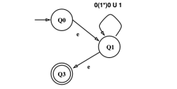
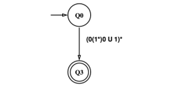
Figure 5. GNFA example

GNFA에서 RE를 얻는 절차는 기저 조건과, 재귀적 단계로 나뉜다. 먼저 기저 조건은 만약 상태가 2개(시작/종료)뿐이면, 답은 [math]\displaystyle{ \delta(q_{start}, q_{accept}) }[/math]이라는 것이다. 이는 시작 상태에서 종료 상태로 전이하는 라벨이 곧 정규표현식이라는 것을 의미한다. 재귀적 단계는 아래와 같다:

1. 파일:Figure 6. Remove Q2.png

   Figure 6. Remove Q2

   파일:Figure 7. Remove Q1.png

   Figure 7. Remove Q1

   상태가 2개 초과라면, 제거할 상태 [math]\displaystyle{ q_{rip} }[/math]을 하나 선택한다. 이때 [math]\displaystyle{ q_{start}, q_{end} }[/math]는 제외한다.
2. [math]\displaystyle{ q_{rip} }[/math]를 제외한 새로운 상태 집합 [math]\displaystyle{ Q' = Q - \{q_{rip}\} }[/math]을 정의한다.
3. 이에 따라 전이 [math]\displaystyle{ \delta }[/math]를 [math]\displaystyle{ \delta'(q_i, q_j) = R_1(R_2)*R_3 \cup R_4 }[/math]와 같이 재정의한다. 이때 [math]\displaystyle{ R_1,R_2,R_3,R_4 }[/math]는 아래와 같다:
   1. [math]\displaystyle{ R_1 = \delta(q_i, q_{rip}) }[/math]
   2. [math]\displaystyle{ R_2 = \delta(q_{rip}, q_{rip}) }[/math] → 자신으로 돌아오는 루프
   3. [math]\displaystyle{ R_3 = \delta(q_{rip}, q_j) }[/math]
   4. [math]\displaystyle{ R_4 = \delta(q_i, q_j) }[/math]

[math]\displaystyle{ q_i }[/math]에서 [math]\displaystyle{ q_j }[/math]로 가는 경우는 [math]\displaystyle{ q_{rip} }[/math]를 거치는 경우와 아닌 경우 두 가지로 나뉜다. 먼저, [math]\displaystyle{ R_4 = \delta(q_i, q_j) }[/math]는 [math]\displaystyle{ q_i }[/math]에서 [math]\displaystyle{ q_j }[/math]로 [math]\displaystyle{ q_{rip} }[/math]을 거치지 않고 전이가 이뤄지는 라벨을 의미한다.

파일:Figure 4. path through q rip.png

Figure 4. path through [math]\displaystyle{ q_rip }[/math]

[math]\displaystyle{ q_{rip} }[/math]을 거쳐서 가는 경우는 figure 4와 같이 표현된다. 따라서 이와 같은 경우에서 읽어들이는 문자열은 [math]\displaystyle{ R_1(R_2)*R_3 }[/math]이다. 따라서 두 경로를 합친 전이 라벨은 [math]\displaystyle{ \delta'(q_i, q_j) = R_1(R_2)*R_3 \cup R_4 }[/math]이다.

Figure 5, 6, 7은 주어진 GNFA에서 정규표현식을 도출하는 예시이다.

Regular Algebra

정규표현식의 연산은 집합 연산의 대수적 성질과 유사하다. 먼저, 합집합에 대한 대수 법칙들은 아래와 같다:

• 교환법칙(Commutative law): [math]\displaystyle{ R_1 \cup R_2 = R_2 \cup R_1 }[/math]
• 결합법칙(Associative law): [math]\displaystyle{ R_1 \cup (R_2 \cup R_3) = (R_1 \cup R_2) \cup R_3 }[/math]
• 항등원(Identity): [math]\displaystyle{ R \cup \empty = R }[/math]
• 멱등법칙(Idempotence): [math]\displaystyle{ R \cup R = R }[/math]

Concatenation과 Kleene star 연산에 대한 대수 법칙들은 아래와 같다:

• 결합법칙(Associative law): [math]\displaystyle{ R_1 \circ (R_2 \circ R_3) = (R_1 \circ R_2) \circ R_3 }[/math]
• 분배법칙(Distributive law): [math]\displaystyle{ R \circ (S_1 \cup S_2) = (R \circ S_1) \cup (R \circ S_2) }[/math]
• 항등원(Identity): [math]\displaystyle{ R \circ \epsilon = R = \epsilon \circ R }[/math]
• 영원소(Zero): [math]\displaystyle{ R \circ \empty = \empty = \empty \circ R }[/math]
• Kleene star 확장: [math]\displaystyle{ R* = \epsilon \cup (R \circ R*) = \epsilon \cup (R* \circ R) }[/math]

이들이 참인 것은 언어의 정의를 사용하여 증명할 수 있다. 예를 들어, [math]\displaystyle{ R \circ \epsilon = R }[/math]은:

[math]\displaystyle{ L(R\circ \epsilon = R) = L(R) \circ L(\epsilon) }[/math]
[math]\displaystyle{  = \{xy|x\in L(R),\,\,y\in L(\epsilon)\} }[/math]
[math]\displaystyle{  = \{x\epsilon | x \in L(R)\} = \{x|x\in L(R)\} = L(R) }[/math]

과 같이 증명된다.

Derivatives of RE

정규표현식의 미분(derivative)는 아래와 같이 정의된다:

언어 [math]\displaystyle{ L \subseteq \Sigma* }[/math], 문자 [math]\displaystyle{ a \in \Sigma }[/math]가 정의되었을 때,
Brzozowski derivative: [math]\displaystyle{ a^{-1}L=\{x|ax \in L\} }[/math]

즉, 언어 L에 속하는 문자열 중, 앞에 a가 붙은 것에서 a를 떼어낸 나머지 부분 집합을 의미한다. 예를 들어 [math]\displaystyle{ L = \{ }[/math]"[math]\displaystyle{ ab }[/math]"[math]\displaystyle{ , }[/math]"[math]\displaystyle{ ac }[/math]"[math]\displaystyle{ , }[/math]"[math]\displaystyle{ aac }[/math]"[math]\displaystyle{ , }[/math]"[math]\displaystyle{ bc }[/math]"[math]\displaystyle{ \} }[/math]를 [math]\displaystyle{ a }[/math]에 대한 미분을 취하면, [math]\displaystyle{ a^{-1}L = \{ }[/math]"[math]\displaystyle{ b }[/math]"[math]\displaystyle{ , }[/math]"[math]\displaystyle{ c }[/math]"[math]\displaystyle{ , }[/math]"[math]\displaystyle{ ac }[/math]"[math]\displaystyle{ \} }[/math]이다. 이때 [math]\displaystyle{ L \subseteq \Sigma* }[/math]이 정규 언어이고 [math]\displaystyle{ a \in \Sigma }[/math]이면 [math]\displaystyle{ a^{-1}L }[/math]도 정규 언어이다.

이때 정규 표현식 R을 문자 a로 미분한 것을 [math]\displaystyle{ \partial_aR }[/math]이라 정의한다. 이때 해당 정의는 재귀적으로 주어진다. 아래는 정규 표현식의 미분 정의이다:

1. [math]\displaystyle{ \partial_ab = \begin{cases} \epsilon, & if\,\,a=b \\ \empty, & otherwise \end{cases} }[/math] [math]\displaystyle{ \rightarrow }[/math] a와 같은 문자면 지워지고 ε, 다르면 공집합
2. [math]\displaystyle{ \partial_a\epsilon = \empty }[/math] [math]\displaystyle{ \rightarrow }[/math] 빈문자열은 시작 문자가 없으므로 매칭 불가
3. [math]\displaystyle{ \partial_a\empty = \empty }[/math] [math]\displaystyle{ \rightarrow }[/math] 공집합은 당연히 미분해도 공집합
4. [math]\displaystyle{ \partial_a(R_1\cup R_2) = \partial_aR_1 \cup \partial_aR_2 }[/math] [math]\displaystyle{ \rightarrow }[/math] 합은 각각 미분 후 합치므로 분배법칙 적용
5. [math]\displaystyle{ \partial_a(R_1R_2) = \begin{cases} (\partial_aR_1)R_2 \cup (\partial_aR_2), & if\,\,\epsilon \in L(R_1) \\ (\partial_aR_1)R_2, & otherwise \end{cases} }[/math] [math]\displaystyle{ \rightarrow }[/math] 연결의 경우, 첫 부분이 ε을 포함하는지에 따라 달라짐
6. [math]\displaystyle{ \partial_a(R_1*) = (\partial_aR_1)R_1* }[/math] [math]\displaystyle{ \rightarrow }[/math] 클리니 스타는 한 번 소비 후 다시 반복 가능

이때 정규표현식을 미분한 뒤 그 언어를 취한 것은 원래 언어의 Brzozowski derivative이다. 이는 아래와 같이 정의된다:

[math]\displaystyle{ L(\partial_aR)=a^{-1}L(R) }[/math]

이때 5번 정의에서 중요한 것은, [math]\displaystyle{ \epsilon \in L(R_1) }[/math] 여부를 판단해야 한다는 것이다. 따라서 빈 문자열이 언어에 속하는지 판별하는 규칙을 재귀적으로 정의해야 하며, 이는 아래와 같다:

• [math]\displaystyle{ \epsilon \notin L(a) }[/math] (단일 문자엔 빈 문자열이 없음)
• [math]\displaystyle{ \epsilon \in L(\epsilon) }[/math]
• [math]\displaystyle{ \epsilon \notin L(\empty) }[/math]
• [math]\displaystyle{ \epsilon \in L(R*) }[/math] (스타는 빈 문자열 항상 포함)
• [math]\displaystyle{ \epsilon \in L(R_1 \cup R_2) \Leftrightarrow \epsilon \in L(R_1) \lor \epsilon \in L(R_2) }[/math]
• [math]\displaystyle{ \epsilon \in L(R_1R_2) \Leftrightarrow \epsilon \in L(R_1) \land \epsilon \in L(R_2) }[/math]

Brzozowski’s Theorem

두 정규 표현식 R과 R'이 congruent하다는 것은, 특정한 대수적 법칙들을 이용해서 서로 같은 언어를 표현한다는 것을 증명할 수 있다는 것이다. 이때 쓰이는 법칙은 정규언어의 합연산([math]\displaystyle{ \cup }[/math])에 대한 기본 성질들이다:

• Idempotence(멱등법칙): [math]\displaystyle{ R \cup R =R }[/math]
• Commutativity(교환법칙): [math]\displaystyle{ R_1 \cup R_2 = R_2 \cup R_1 }[/math]
• Associativity(결합법칙): [math]\displaystyle{ (R_1 \cup R_2) \cup R_3 = R_1 \cup (R_2 \cup R_3) }[/math]

Brzozowski’s Theorem은 아래와 같다:

Every regular expression [math]\displaystyle{ R }[/math] has at most finitely many non-congruent derivatives. 
These form the set of states of a DFA that recognizes [math]\displaystyle{ L(R) }[/math].

이는 어떤 정규 표현식 [math]\displaystyle{ R }[/math]을 계속 미분해 나가면 새로운 정규표현식들이 생기지만, 하지만 동치 관계(congruence)를 고려하면 사실 서로 다른 표현식은 유한 개만 존재한다는 것이다. 즉, 어떤 한 정규표현식으로부터 미분하여 얻을 수 있는 "비동치(non-congruent)" derivative는 유한 개뿐이라는 뜻이다. 예를 들어, 아래는 서로 다르게 보이는 언어들이 사실 동치인 언어라는 것을 보여준다.

• [math]\displaystyle{ R\cup \empty = R }[/math]
• [math]\displaystyle{ R \empty = \empty }[/math]
• [math]\displaystyle{ \empty R = \empty }[/math]
• [math]\displaystyle{ R\epsilon = R }[/math]
• [math]\displaystyle{ \epsilon R = R }[/math]

위의 성질을 이용하면, 미분 과정에서 생긴 복잡한 정규표현식들을 간단히 축약할 수 있다.

Obtaining a DFA from a Regular Expression

Brzozowski 미분을 사용하면 어떤 정규표현식이 나타내는 DFA를 직접적으로 구성할 수 있다. 이는 아래의 절차를 가진다:

1. 상태 집합 [math]\displaystyle{ Q }[/math]를 정규표현식 자체만을 포함하는 [math]\displaystyle{ \{R\} }[/math]로 시작한다.
2. 아직 탐색되지 않은 표현식 [math]\displaystyle{ E \in Q }[/math]에 대해, 각 문자 [math]\displaystyle{ a \in \Sigma }[/math]로 미분 [math]\displaystyle{ \partial_aE }[/math]를 계산한다.
   • 새로운 표현식이 기존 것과 동치(congruent)하지 않다면 [math]\displaystyle{ Q }[/math]에 추가한다.
   • 해당 과정은 Brzozowski 정리에 의해 유한 단계에서 종료된다.
3. Initial state: [math]\displaystyle{ q_0 = R }[/math]
4. Accept states: [math]\displaystyle{ \epsilon \in L(E) }[/math]를 만족하는 표현식 [math]\displaystyle{ E \in Q }[/math]를 accept 상태로 둔다.
5. 전이 함수 [math]\displaystyle{ \delta }[/math]: [math]\displaystyle{ \delta(E, a) = E_a }[/math]. 이때 [math]\displaystyle{ E_a = \partial_aE \in Q }[/math]

이를 통해서 DFA [math]\displaystyle{ = (Q,\Sigma,\delta, q_0,F) }[/math]가 완전히 정의된다. 이를 적용한 예시는